This dashboard provides real-time indicators of US labor market and business cycle conditions. It starts with three core labor market indicators: the unemployment rate, vacancy rate, and labor market tightness. These metrics jointly characterize the functioning of the labor market. The dashboard also plots the Beveridge curve, which relates the unemployment and vacancy rates.
From these, the dashboard calculates two metrics that quantify how far the labor market is from social efficiency: the full-employment rate of unemployment (FERU) and the unemployment gap. These two metrics are key determinants of optimal monetary policy and fiscal policy.
Finally, the dashboard presents two metrics derived from the Michez rule—a new, fast, and robust method to detect recessions. The recession indicator and recession probability highlight early signs of labor market weakening and signal upcoming deterioration.
All charts automatically update as new data become available on FRED, providing a real-time view of the US business cycle.
Key events
- November 2025 - The US government was shut down between 10/01/2025 and 11/12/2025, which seriously affected the collection of labor market data. The September 2025 wave of the Current Population Survey (CPS)—which is the source of the unemployment and labor force numbers—was collected normally but published late, on 11/20/2025. The October 2025 wave of the CPS was not collected and will not be collected retroactively. So there will be no unemployment and labor force estimates for October 2025. Accordingly, the dashboard will not provide data for October 2025.
- September 2025 - The Federal Reserve cuts the federal funds rate by 25 basis points in response to the cooling of the labor market.
- August 2025 - The US labor market dips below full employment for the first time since April 2021.
- May 2025 - The dashboard is live.
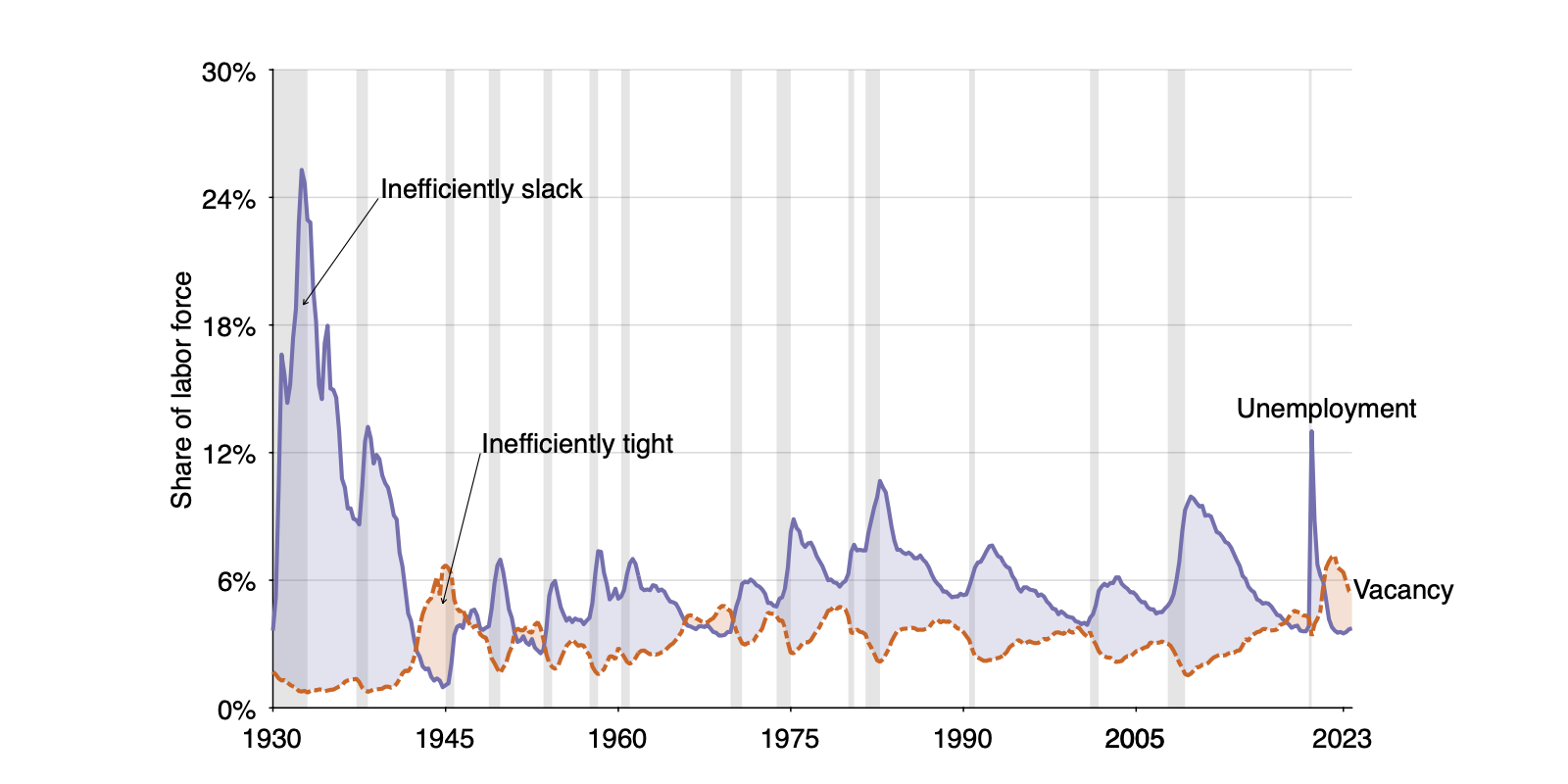
US unemployment rate
- Construction: The unemployment rate is the number of job seekers divided by the number of labor force participants.
- Interpretation: The unemployment rate measures the share of people who have not succeeded in finding a job, among all those who are able and willing to work. This is the standard, official unemployment rate (U3).
- Source: The numbers of job seekers and labor force participants are measured by the US Bureau of Labor Statistics (BLS) from the Current Population Survey (CPS), which is a large-scale household survey.
- Download unemployment rate
- View unemployment rate in full screen
US vacancy rate
- Construction: The vacancy rate is the number of job openings divided by the number of labor force participants.
- Interpretation: The vacancy rate measures the number of job openings per labor force participant.
- Source: The number of job openings is measured by the BLS from the Job Openings and Labor Turnover Survey (JOLTS), which is a large-scale firm survey.
- Download vacancy rate
- View vacancy rate in full screen
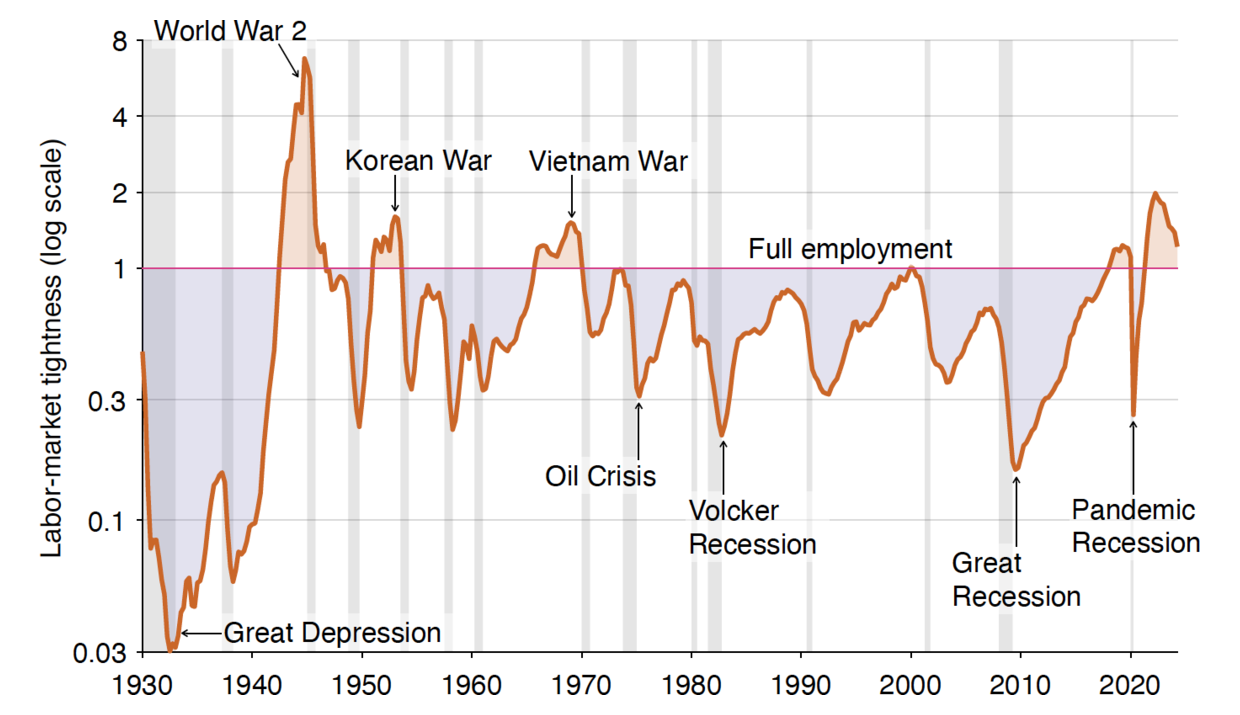
US labor market tightness
- Construction: Labor market tightness is the vacancy rate divided by the unemployment rate.
- Interpretation: Labor market tightness measures the number of job openings per job seeker. A tightness of 1 marks full employment, or equivalently labor market efficiency. When tightness is below 1, the labor market is inefficiently slack. When tightness is above 1, the labor market is inefficiently tight.
- Download labor market tightness
- View labor market tightness in full screen
US Beveridge curve
- Construction: The Beveridge curve links the unemployment rate to the vacancy rate.
- Interpretation: During typical business cycles, the economy moves along a stable Beveridge curve. In recessions the unemployment rate increases while the vacancy rate decreases; in expansions the unemployment rate decreases while the vacancy rate increases. The labor market is at full employment whenever the unemployment and vacancy rates are equal. Hence, the labor market is inefficiently tight whenever the Beveridge curve is above the 45° ray and inefficiently slack whenever the curve is below the 45° ray.
- View Beveridge curve in full screen
US full-employment rate of unemployment (FERU)
- Construction: The full-employment rate of unemployment (FERU) is the geometric average of the unemployment and vacancy rates: $u^\ast = \sqrt{u \times v}$, where $u$ is the unemployment rate, $v$ is the vacancy rate, and $u^\ast$ is the FERU.
- Interpretation: The FERU marks full employment and, by construction, labor market efficiency. So the FERU is also the socially efficient unemployment rate.
- Visualization: On the Beveridge diagram, the FERU is at the intersection of the Beveridge curve and the 45° ray. The implication is that the FERU is determined by the location of the Beveridge curve: it is higher whenever the Beveridge curve is further outward.
- Download FERU
- View FERU in full screen
US unemployment gap
- Construction: The unemployment gap is given by $u - u^\ast$, where $u$ is the unemployment rate and $u^\ast$ is the FERU.
- Interpretation: The unemployment gap indicates the distance from full employment. A positive gap marks an inefficiently slack labor market. A negative gap marks an inefficiently tight labor market.
- Download unemployment gap
- View unemployment gap in full screen
US recession indicator
- Construction: The recession indicator is the minimum of an unemployment indicator (the increase in the 3-month average of the unemployment rate above its 12-month low; used in Sahm rule) and a vacancy indicator constructed analogously (the decrease in the 3-month average of the vacancy rate below its 12-month high).
- Interpretation: The Michez rule signals a recession when the recession indicator crosses the threshold of 0.29pp.
- Download recession indicator
- View recession indicator in full screen
US recession probability
- Construction: The recession probability is computed from the dual-threshold extension of the Michez rule. The recession probability is the fraction of the 0.29pp–0.81pp band that the recession indicator has covered: $p =$ (indicator $-$ 0.29) $/$ (0.81 $-$ 0.29).
- Interpretation: The dual-threshold Michez rule works as follows: values of the indicator between 0.29pp and 0.81pp signal a probable recession; values above 0.81pp signal a certain recession. This dual-threshold extension accounts for uncertainty in the true recession threshold and provides a simple way to nowcast recession risk.
- Download recession probability
- View recession probability in full screen
- Note: This is not the recession probability computed in more recent work and covered by the Financial Times. The new recession probability will only be added to the dashboard once the method is finalized. The newer method estimates a higher recession probability in 2025 (64% in September 2025) because it discounts temporary dips in recession indicators.
Frequently asked data questions
When do the numbers for the current month become available?
The data required to populate the dashboard for a given month are released by the BLS in the first week of the following month, usually on a Tuesday for the JOLTS data and on a Friday for the CPS data:
- Latest JOLTS data release
- Latest CPS data release
Accordingly, the dashboard usually provides a complete picture for the current month on the first Friday of the following month. The schedule of future data releases is announced well in advance by the BLS.
The JOLTS data for a given month appear to be released one month after the CPS data for the same month, but to best align labor force and vacancy data, we shift forward by one month the number of job openings from JOLTS. For instance, we assign to April 2025 the number of job openings that the BLS assigns to March 2025. The motivation for this shift is that the number of job openings from the JOLTS refers to the last business day of the month (Monday 31 March 2025 in our example), while the labor force from the CPS refers to the Sunday–Saturday week including the 12th of the month (Sunday 6 April 2025–Saturday 12 April 2025 in our example). So the number of job openings refers to a day that is closer to the next month’s CPS reference week than to the current month’s CPS reference week. In our example, the CPS survey for April started in the same week as the JOLTS survey for March.
Are the numbers final upon release? Or will they be revised?
The numbers constructed in real time might not be final because the unemployment, vacancy, and labor force data are revised by the BLS after their initial release:
- The number of job openings released by the BLS is preliminary and updated one month after its initial release, to incorporate additional survey responses received from businesses and government agencies and from the recalculation of seasonal factors.
- The BLS revises the prior five years of CPS and JOLTS data each year at the beginning of January, to account for revisions to seasonal factors, population estimates, and employment estimates.
Yet, revisions to labor market data are generally minimal, especially compared to GDP revisions, so the information provided in real time by labor market data is generally indistinguishable from the information provided in the final version.
Is the unemployment rate the same as the BLS unemployment rate?
Yes, almost. The two unemployment rates are computed similarly, but the BLS reports the unemployment rate with one-digit precision, while the dashboard reports it with two-digit (basis-point) precision. This higher precision is useful for recession detection, as recession indicators are computed and reported at the basis-point level.
Is the vacancy rate the same as the BLS vacancy rate?
No. The BLS computes the vacancy rate as the number of job vacancies divided by the number of employed workers plus job openings. This computation is problematic for two reasons. First, it means that the BLS unemployment and vacancy rates are not consistent with each other, since one uses the number of employed workers plus unemployed workers in the denominator, while the other uses the number of employed workers plus job openings in the denominator. Second, the BLS vacancy rate is not a useful variable in labor market matching models.
By contrast, the dashboard computes the vacancy rate as the number of job vacancies divided by the number of employed workers plus unemployed workers. Our unemployment and vacancy rates are consistent with each other. Furthermore, our vacancy rate is the variable that appears directly in labor market matching models.
Isn’t the vacancy rate inflated by ghost job postings?
Vacancy data have recently been criticized for being polluted by ghost or fake vacancies. These vacancies do not actually represent an open position, and will not lead to a new hire. A recent article by CBS News explains that fake job listings are a growing problem in the labor market. Employ America has gone one step further and argued that vacancy numbers are vacuous in general and should never be used by policymakers. Let’s go over the various criticisms raised by such pieces and address them.
Aren’t vacancies poorly measured?
A first claim is that vacancy numbers are polluted by ghost vacancies. But vacancies are measured by the BLS, just like all other labor market statistics; they are not measured from online job postings.
Specifically, the JOLTS asks firms to report the number of vacancies that they currently have, where a vacancy is defined as follows:
- A specific position exists and work is available.
- The job could start within 30 days.
- The firm is actively recruiting workers from the outside to fill the position.
These questions are similar to the questions asked by the BLS to workers in the CPS in order to assess their labor force status. To be classified as a job seeker, a respondent must confirm that:
- They do not currently work but are willing to work.
- They are available to start work immediately.
- They have been actively searching for a job in the last four weeks.
The threshold for reporting a vacancy is the same as the threshold for reporting being unemployed. The firm and the worker have to answer that they have been actively searching on the labor market—for instance through online job portals.
Isn’t it exceedingly easy to post vacancies on online job boards?
A second point relates to online job boards: it is very easy for firms to list job advertisements online, so the number of online job postings might not be meaningful. As noted above, however, our vacancy numbers do not come from online job boards: they are measured by the BLS through JOLTS. So what happens on online job boards is irrelevant.
In fact, the internet and online job portals might not have much effect on the job market. Looking at the academic job market, it does not seem that the amount of time and effort required to recruit colleagues is appreciably diminished by online job portals. Most of the recruiting time is spent on four things: reading applications and papers; interviewing candidates; flying out candidates; and debating with colleagues. None of these four tasks are affected by online job boards.
Don’t firms post more than one vacancy per hire?
A third supposed issue is that firms post more than one vacancy per hire—which leads some to believe that some vacancies are fake since they do not result in a hire. But this is exactly how firms behave in matching models! In these models, if a firm wants to recruit one worker this month but knows that a vacancy is only filled with probability 1/3, then the firm will post 3 vacancies to hire one worker in expectation.
The key point is that in matching models, vacancies do not represent actual positions but recruiting effort—an effort to try to find workers through the matching process. This is also what vacancies represent in reality, as ZipRecruiter’s Julia Pollak explains in the CBS article:
When you have fewer candidates per opening, you have to be more creative. The high openings figure does partly reflect recruiting intensity, and not actual roles and seats and slots.
The bottom line is firms behave in reality exactly as in the model. The fact that firms post several vacancies per position does not mean that vacancy data should be discounted. This behavior is what matching models predict.
Aren’t vacancies just noise?
Another complaint is that vacancy numbers are just too noisy to be helpful. But the US vacancy and unemployment rates are strongly negatively correlated, moving along a downward-sloping Beveridge curve. The Beveridge curve is one of the most robust macro relationships—how would it arise if vacancy numbers were just noise?
Given that unemployment and vacancies come from two entirely different sources—a firm survey (JOLTS) and a household survey (CPS)—it is striking that they comove so closely. Furthermore, the information conveyed by vacancies is consistent with other measures of the state of the US labor market. Labor market tightness—which is the ratio of the vacancy rate and unemployment rate—indicates that the US labor market has been inefficiently tight only on four occasions: during World War 2, the Korean War, the Vietnam War, and the coronavirus pandemic. An analysis of 25 million newspaper articles by Caldara, Iacovello, and Yu identifies the same periods as marked by severe labor shortages. So our vacancy measure matches well with broader indicators of labor market tightness and the public’s experience.
Why are fake vacancies an issue now?
Firms have been posting vacancies for a century at least, so why do vacancies only appear fake now? The reason is that in 2022–2024, the labor market was exceptionally tight: the tightest it had been since the end of World War 2. Such exceptional tightness means that vacancies are filled at the slowest rate in the postwar period. Indeed, in a tight market, job seekers find jobs at a high rate, but firms fill vacancies at a slow rate—as predicted by matching models.
Because vacancies are filled at such a slow rate, the number of vacancies posted for one actual position has exploded—reinforcing the impression of fake vacancies. But this was expected: this is exactly what matching models predict. Firms post several vacancies per position because they realize that the yield of each vacancy is low.
Conclusion
Although vacancies are not discussed much in the macro literature, there is an old and large literature that studies vacancies and explains how to measure them. In fact that literature is as old as the literature studying unemployment, going back to the work of Beveridge in 1944, Rees in 1957, Abraham in 1983 and in 1987, and Zagorsky in 1998. Modern research on job vacancies include work by Barnichon in 2010 and Petrosky-Nadeau and Zhang in 2021.
What is the shape of the Beveridge curve?
The Beveridge curve is approximately a rectangular hyperbola: $u \times v = A$, where $A>0$ is a constant that determines the location of the curve. This is apparent once the Beveridge curve is plotted on log scale: it traces a line of slope -1, shifting every decade or so.
The hyperbolic shape implies that unemployment and vacancy rates are not only negatively related, but inversely related. So when the vacancy rate falls by $x$%, the unemployment rate will increase by $x$%. And when the vacancy rate increases by $x$%, the unemployment rate will decrease by $x$%.
There is a view that the Beveridge curve might have an unusual shape in the aftermath of the pandemic. Part of the issue is that the Beveridge curve shifted very far out in 2020, when the labor market was shattered by the coronavirus, and then between 2022 and 2023, the curve became almost vertical. But the appearance of verticality can be explained by the fact that the Beveridge curve was returning to its old location while the labor market was cooling.
In the last 2 years, the Beveridge curve is almost back to a rectangular hyperbola. In April 2023, the reading was $u =$ 3.45% and $v =$ 5.74%. In April 2025, the reading is $u =$ 4.19% and $v =$ 4.20%. So $v$ decreased by [5.74 $-$ 4.20] $/$ 5.74 $=$ 26.8% while $u$ increased by [4.19 $-$ 3.45] $/$ 3.45 $=$ 21.4%. A hyperbola says that $u$ should have increased by 26.8% instead of 21.4%. So the curve is slightly steeper than a hyperbola, but is not far off. The elasticity of the curve is 26.8% $/$ 21.4% $=$ 1.25 instead of 1.
How does the Michez rule relate to the Sahm rule?
The Michez rule is based on the same idea as the Sahm rule: looking for a rapid deterioration of labor market variables to detect recessions. But while the Sahm rule only uses the unemployment rate for detection, the Michez rule uses both the unemployment and vacancy rates.
By combining data on unemployment and vacancies, the Michez rule obtains a less noisy signal of recessions, so it can detect recessions faster than the Sahm rule:
- Average detection delay, 1960–2021: 1.2 months < 2.7 months
- Maximum detection delay, 1960–2021: 3 months < 7 months
The Michez rule is also more robust: it identifies all 15 recessions since 1929 without false positives, whereas the Sahm rule breaks down before 1960.
Do the dashboard statistics apply to other countries?
Unemployment rate, vacancy rate, and labor market tightness can be computed in the same way in other countries in which similar raw data (number of job seekers, number of job vacancies, number of labor force participants) are available.
The FERU formula $u^\ast = \sqrt{uv}$ does require assumptions on the cost of unemployment, cost of recruiting, and shape of the Beveridge curve. In countries in which the unemployment and recruiting costs and the shape of the Beveridge curve are different than in the United States, the FERU must be computed from a more general formula.
The Michez-rule recession indicator can be computed for any country, but the recession threshold of 0.29pp needs to be recalibrated. The value of 0.29pp is the lowest threshold that generates no false positives in the United States between 1960 and 2021. In other countries, the recession indicator will take different values, and recessions will occur at different times, so the threshold will have to be recomputed.
Similarly, the upper threshold of 0.81pp used in the dual-threshold Michez rule to infer a recession probability will have to be recalibrated in other countries. The value of 0.81pp is the highest threshold that generates no false negatives in the United States between 1960 and 2021. In other countries, the recession indicator will take different values, and recessions will occur at different times, so the threshold will have to be recomputed. Once the thresholds are recalibrated, the recession probability can be computed using a similar formula.
Frequently asked policy questions
What is full employment?
The federal government and Federal Reserve are mandated to maintain the economy at full employment, or maximum employment. (The two terms have been used interchangeably.) This legislative mandate comes from the Employment Act of 1946, the Federal Reserve Reform Act of 1977, and the Full Employment and Balanced Growth Act of 1978 (known informally as the Humphrey–Hawkins Act).
The issue is that these texts do not explain what full employment is. The Humphrey-Hawkins Act did set an unemployment target of 3% within 5 years of the law (and 4% for young workers). But these numbers were never taken seriously, in part because policymakers rightly understood that the full-employment unemployment rate could not be a fixed number. When testifying in front of Congress in 1975 in his capacity of chair of the CEA, Alan Greenspan was asked what the target for full employment should be. He responded:
I do not think we should set a target.
But the Employment Act and Full Employment and Balanced Growth Act clearly state that achieving full employment is a way to maximize social welfare. So we translate full employment as social efficiency. Accordingly, we compute the FERU as the unemployment rate that achieves a socially efficient allocation of labor. This allocation maximizes social output by minimizing the uses of labor that are socially unproductive: both jobseeking and recruiting. The computation yields the formula $u^\ast = \sqrt{uv}$.
Does the FERU formula hinge on the presumption that vacancies are unmet labor demand?
No. A common misunderstanding is that our analysis treats JOLTS job openings as a measure of unmet labor demand.1 This is not the case. Nowhere in the analysis do we interpret vacancies that way. Beveridge did interpret job vacancies as unmet labor demand and accordingly defined full employment as the point where job vacancies exceed job seekers. But our approach is different: we interpret vacancies as an indirect measure of the labor devoted to recruiting. In the United States, it takes roughly one recruiter to handle one vacancy, so the number of vacancies tracks the amount of labor devoted to recruiting. This empirical regularity is what we use in deriving the FERU.
Is the FERU the same as the NAIRU?
No. In recent times, the US government has used the non-accelerating-inflation rate of unemployment (NAIRU) as full-employment target. For instance, the Joint Economic Committee recently wrote:
Today, full employment is considered by many to be synonymous with the non-accelerating inflationary rate of unemployment (NAIRU)—the rate of unemployment that neither stokes nor slows inflation.
Similarly, in 2024, the Council of Economic Advisers described the concept of full employment as follows:
Modern economics has generally defined full employment by citing the theoretical concept of the lowest unemployment rate consistent with stable inflation, which is referred to as $u^\ast$, the non-accelerating inflationary rate of unemployment (termed NAIRU).
These quotes are particularly meaningful because the Joint Economic Committee and Council of Economic Advisers were both created by the Employment Act of 1946 to ensure that the government achieved its full-employment mandate.
But this is a misconception: the NAIRU is an entirely different concept than the FERU. The FERU is the socially efficient unemployment rate. The NAIRU is the unemployment rate at which inflation remains stable. Since there is no guarantee that the unemployment rate prevailing under stable inflation is efficient, there is no guarantee that the NAIRU and FERU are the same.
Is the FERU the same as the CBO’s NRU?
Another full-employment target used by the US government is the natural rate of unemployment (NRU)—recently rebranded noncyclical rate of unemployment—constructed by the Congressional Budget Office (CBO). The CBO’s NRU is a slow-moving trend of the unemployment rate computed by assuming that the labor market was at full employment in 2005 and then incorporating changes in the demographic composition of the labor force over time.
But, without a theory of full employment, it is impossible to know whether the US labor market really was at full employment in 2005, and by induction, whether the NRU in any year measures full employment. The NRU can therefore not be a satisfactory measure of full employment.
Why is the FERU not constant?
The FERU is computed as the unemployment rate that maximizes social welfare, or equivalently that minimizes the nonproductive use of labor: both unemployment and recruiting. As it takes one worker to service one job vacancy, the nonproductive use of labor is measured by the number of job seekers and job vacancies. Through the Beveridge curve, the numbers of job seekers and vacancies are inversely related, so it is not possible to reduce the numbers of job seekers and job vacancies at the same time. Instead the social planner faces a tradeoff which is resolved by the FERU.
Because the FERU describes the socially efficient position of the labor market on the Beveridge curve, it is not constant but determined by the location of the Beveridge curve. When the Beveridge curve shifts outward, the FERU increases; when the Beveridge curve shifts inward, the FERU decreases. Typical Beveridge curve shifts do not affect the FERU much. For instance, between 1951 and 2019, the FERU remained between 3.1% and 5.5%, with an average value of 4.3%. The Beveridge curve did shift in and out during the postwar period, but the shifts were not large enough to produce noteworthy changes in the FERU.
During the coronavirus pandemic, the Beveridge curve shifted out dramatically. The Beveridge curve then slowly shifted back inward. In 2025, the curve is almost back to its pre-pandemic position, although it remains somewhat further out. The dramatic shift raised the FERU significantly: from 3.8% in January 2020 to 7.5% in April 2020. As the Beveridge curve normalized in the years after the pandemic, the FERU returned to normal levels. The FERU increase that followed the pandemic is extraordinary: such a large increase had never been recorded before. The pandemic was also the first time in the past century that the FERU crossed 6%.
What does a positive unemployment gap imply for monetary policy?
Targeting the FERU and setting the unemployment gap to zero is required by the Federal Reserve’s legal mandate. So by that mandate, the Fed should lower interest rates any time the unemployment gap is positive to stimulate the economy and labor market.
Furthermore, maintaining the unemployment gap at zero is the optimal monetary policy in a range of monetary models built around the Beveridge curve. For instance, in a model in which inflation is fixed, the optimal monetary policy is to adjust interest rates in order to maintain unemployment at the FERU. In such a model, monetary policy does not affect inflation, so it is optimal to keep unemployment at the FERU.
Of course fixed inflation is a strong assumption. But maintaining unemployment at the FERU is also optimal in models with endogenous inflation, as long as the divine coincidence holds. In such models, lower unemployment leads to higher inflation. But when the unemployment rate is efficient, inflation is on target, so there is no trade-off between inflation and unemployment. Maintaining unemployment at the FERU also maintains inflation on target, so it is the optimal policy.
How big should adjustments in interest rates be to keep the economy at full employment? The US monetary multiplier—the unemployment-rate decrease achieved by lowering the nominal interest rate by 1pp—is estimated to be around 0.5. Hence, the Fed should cut its interest rate by 1/0.5 = 2pp for each positive percentage point of unemployment gap; it should raise its interest rate by 2pp for each negative percentage point of unemployment gap.
Even when the divine coincidence does not hold, the Fed should use the unemployment gap to adjust the federal funds rate. When the divine coincidence fails, monetary policy faces a tradeoff between closing the unemployment gap and bringing inflation to its target, so targeting the FERU is no longer optimal. Nevertheless, the optimal interest rate depends on the FERU: it is determined by weighing the unemployment gap against the inflation gap. Indeed, the optimal unemployment and inflation gaps are related by:
$$\frac{u - u^\ast}{\pi - \pi^\ast} = \frac{\beta}{\alpha},$$
where $\alpha$ measures the welfare cost of unemployment relative to inflation, and $\beta$ measures the response of inflation to unemployment through the Phillips curve.
If unemployment is particularly costly (high $\alpha$) or if the Phillips curve is flat (low $\beta$), the optimal unemployment gap is small relative to the optimal inflation gap. In such cases, the optimal unemployment rate remains close to the FERU, either due to the high marginal cost of unemployment (high $\alpha$) or the limited marginal benefit of unemployment (low $\beta$).
What does a positive unemployment gap imply for fiscal policy?
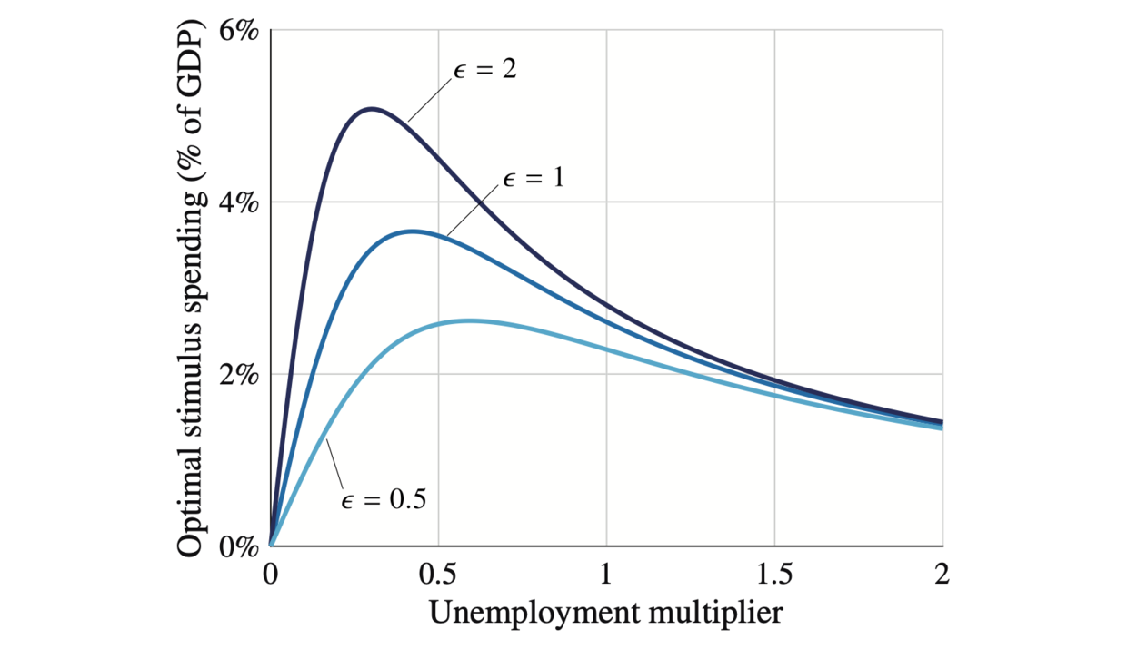
Fiscal policy should also be adjusted to reduce the unemployment gap. In fact, optimal stimulus spending—the amount of public spending above the spending given by the Samuelson rule—can be expressed as a function of three sufficient statistics: unemployment gap (once again), elasticity of substitution between public and private goods (measuring the value of public goods), and the unemployment multiplier (reduction in unemployment from public expenditure). Empirical evidence for the United States suggests that the elasticity of substitution is positive and the unemployment multiplier is positive.
The formula and evidence provide several insights:
- The Samuelson rule—which was derived in a neoclassical economy—remains valid in an economy with unemployment as long as unemployment is efficient.
- If unemployment is above the FERU, then public spending should be above the Samuelson rule. That is, stimulus spending should be positive if the unemployment gap is positive.
- Conversely, if unemployment is below the FERU, then public spending should be below the Samuelson rule.
- Optimal stimulus spending is larger when the initial unemployment gap is larger.
- Optimal stimulus spending is larger when the elasticity of substitution between public and private goods is larger. This is because public goods replace private goods better in that case, so public spending is less distortionary.
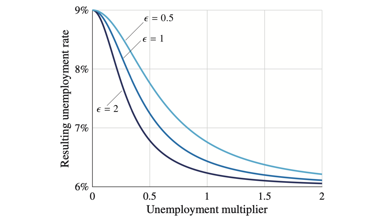
- Maybe unexpectedly, optimal stimulus spending is a hump-shaped function of the unemployment multiplier. Optimal stimulus spending is zero for a zero multiplier, increasing in the multiplier for small multipliers, largest for a moderate multiplier, and decreasing in the multiplier beyond that. So larger multipliers do not necessarily mean larger stimulus spending. The reason is that when public spending becomes more powerful, less of it is required to reduce the unemployment gap.
- With public spending it is optimal to reduce but not eliminate the unemployment gap.
What does a positive unemployment gap imply for matching policies?
When recessions occur, and the unemployment rate rises, it’s typical to hear economists advocate for policies that improve search and matching on the labor market: investment in placement agencies, development of programs to help workers find the right firms, or harsher monitoring of workers’ search effort. This is because all unemployment is frictional in standard models of the labor market, so the natural reflex is to fight search-and-matching frictions.
However, as soon as we move away from the assumption that all unemployment is frictional and make the assumption that part of unemployment is caused by a lack of job, we realize that this is not good policy advice. Indeed, in a model with both job rationing and search-and-matching frictions, frictional unemployment shrinks in slumps, so there is very little scope for policies that improve search and matching.
What does a positive unemployment gap imply for unemployment insurance?
The unemployment gap is not directly useful to compute optimal unemployment insurance (UI) because UI affects workers’ search effort and in effect shifts the Beveridge curve. On the other hand, the tightness gap—the gap between actual and efficient tightness—is a key sufficient statistic for optimal UI. But the efficient tightness is not simply 1 in a world with imperfect consumption insurance: it is given by a more complex formula that involves risk aversion and the consumption drop upon unemployment. So while the tightness gap displayed here gives an indication about required adjustments to UI, a more sophisticated tightness gap must be computed to obtain the optimal UI over the business cycle.
References
- Pascal Michaillat and Emmanuel Saez. 2024. “u* = √uv: The Full-Employment Rate of Unemployment in the United States.” Brookings Papers on Economic Activity 55 (2): 323–390.
- This paper argues that the legal term “full employment” should be translated to “social efficiency” in the economics language.
- The paper then obtains the formula for the US FERU: $u^\ast = \sqrt{uv}$.
- The formula implies that the economy is at full employment when there are as many job seekers as job vacancies; inefficiently tight when there are fewer job seekers than job vacancies; and inefficiently slack when there are more job seekers than job vacancies.
- View the paper
- Pascal Michaillat and Emmanuel Saez. 2025. “Has the Recession Started?” Oxford Bulletin of Economics and Statistics 87 (6): 1047–1058.
- This paper develops the Michez rule, which uses the recession indicator and a threshold of 0.29pp to detect US recessions in real time.
- The paper also proposes a dual-threshold extension of the Michez rule, from which the recession probability is computed.
- View the paper
One of the discussants of our FERU paper for instance makes that assertion. He argues that our analysis is erroneous because it assumes that JOLTS job openings measure the level of unmet labor demand. We never made that assumption, however, and it’s unclear why the discussant thought we did. ↩︎